Figuring a Telescope Mirror

You’ve been polishing on your mirror, which should have produced a spherical mirror. You have checked it for astigmatism, and it is OK if you are at this point. There is a section on Ronchi testing, and if you went forward and checked it over, you know that you can see some turned down edge [TDE] easily with the Ronchi test. Let’s assume that you have done that and your mirror is without TDE.

At this point your mirror should be spherical, not astigmatic, no turned-down edge, completely polished, smooth, scratch-free and ready to parabolize. In this section we’ll talk about the strokes and methods of altering zones toward a paraboloid, and discuss the logic of the tests, such as the Foucault and Caustic Tests. In this section will be very brief discussions regarding these tests.

Basically, the radius of curvature [ROC] for a sphere is the same everywhere on that sphere, while for a paraboloid, it is shorter near the center of the mirror than it is on the outskirts of the mirror. We perform strokes with the polishing lap to shorten the ROC near the center while not shortening the ROC near the edge, with the transition between them smoothly transitioning. Using the Foucault test, we will determine where the mirror is in need of this correction, and address those areas with strokes. We will work parabolizing strokes, then test the mirror to measure our progress, then work the mirror, then test the progress, and on and on until the mirror’s tested condition is within our specifications of being a paraboloid. We will never have a perfect paraboloid, but we will get close enough that the error is acceptable.

Imagine yourself at the center of a spherical ball whose inside is a mirrored surface. Everywhere you look, you’d see yourself. Now if the ball weren’t complete, but rather only a piece of the sphere, then you could still exist at the center of curvature of that spherical segment, and again when you looked into that segment, you’d see yourself. A telescope mirror starts out being spherical on the polished side. Let’s use a 12” f/6 spherical mirror. It has a focal length of 12 times 6 equals 72”. The radius of curvature is twice the focal length, so that’s 144”. If you stood back from the surface of this mirror 144”, you’d be at the center of curvature of that sphere. Since this glass reflects light, then you could move closer to the sphere and see yourself in the glass reflecting back. Holding a flashlight into it helps. Move the light right, the image appears to go right. Now if you move backwards from this surface, eventually you will notice that it goes blurry, and if you keep moving back, you will eventually see yourself up—side-down. If you move your flashlight right, it appears to go left. Moving it up makes it look like you’re moving it down. You have gone past the center of curvature of the sphere. At the point where things go from being “right” to being “inverted” is the center of curvature of this sphere. That is where you test apparatus will go when testing your mirror.

We set up a test jig so that it has the following features: A box with a light in it [I use an LED] with a hole drilled into the plate to let the light shine toward the mirror, a long razor blade that cuts the hole in half so the light looks like a half-Moon, the razor is long enough to point up to the sky and allows me CAREFULLY place my eyeball by it and look past it, longitudinal movement [to and from the mirror] with a measuring device to know its position [a micrometer], and the ability to move the jig transversally [I also use a micrometer, not shown in illustration]. The micrometers are forced into the jig with springs so that it operates as a push-pull system.

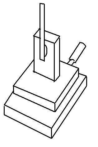
Here is a crude diagram of a test jig. The razor is tall enough to half cover a hole with an LED behind it as well as allow the user to look past the razor. Careful not to cut your cornea, they don’t get fixed. The micrometer enables the positioning and measurement of the apparatus.

Place the mirror on an adjustable test stand. You should be able to physically move the mirror forward and back, as well as tilt and turn it. The test stand should not affect the shape of the mirror, and I mean to the millionths of an inch. So check out the test stand link. The distance between the mirror and the test jig needs to be adjustable, and this can be done by moving the mirror, moving the test jig, or both. Stand behind the test jig and look past it at the mirror. You need to be able to see the light from the test jig reflecting off of the mirror and passing by the sharp side of the razor. Adjust items until this is true. Now move your eyeball closer and closer to the razor. As your eye gets near the razor the entire mirror needs to appear illuminated by this light. If this happens before you get to the razor, then the mirror and test jig are too close together. If you can’t get it to happen, then they are too far apart. Make adjustments until this is satisfied.

When the entire mirror can be illuminated while looking at it past the razor, then you are close. Transversally move the razor so the mirror appears to have a shadow moving into it. This is the light being blocked by the razor as it passes by it on the way to your eyeball. If the shadow moves into the mirror on the same side that the razor is on, then the razor is a bit too close to the mirror and the adjustment needs to move it back from the mirror. If the shadow moves into the mirror on the opposite side that the razor is on, then the razor is a bit too far from the mirror and that adjustment needs to move it forward toward the mirror. However, when the entire mirror appears to fade into darkness simultaneously, then the razor and the light source system is at the center of curvature, right where you want it to be. Practice this, spend a lot of time examining these positions, and spend a lot of time examining the image when you are at the right spot. Get familiar with this process, the image, the ability to make micro-adjustments. This time and this learning will reward you on this and future mirrors. Here is an illustration that might help.

Below is a shadowgram taken with the knife-edge right at the radius of curvature of a nearly spherical mirror. The mirror has a small amount of correction if you look carefully. Also you can see the heat rising off the lower right safety clip. The test is so sensitive that if there is air of a different temperature between the mirror and the test stand, the light will take a slightly different path as it passes through the disturbed air, making itself apparent in the shadowgram. This is a 24” f/3.6.

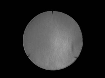
The mirror is spherical if the entire illumination in the mirror fades away uniformly. You may see places on the mirror that don’t fade away with the rest of the mirror. You will be able to see the texture on the glass that appears thousands of times larger than they actually are. Texture with an amplitude of a millionth of an inch can be seen with this apparatus. If you use your polishing process to make this illusion perfectly neutral [null], then you will have a spherical mirror with extreme precision.

There are a few things to look for at this time. Micro-ripple otherwise known as dog biscuit, is the texture roughness that you can see. Even though it may allow the mirror to have a peak to valley acceptable level, it increases you RMS, root mean square, which distributes light outside of the targeted “Airy disk”, which we’ll talk about later. Make your mirror smooth. The bright ring right at the edge of the mirror is a turned down edge. This occurs when polishing with long strokes, and some other things, where the pitch lap forces itself to work the very edge of the mirror and work it down harder than the rest of the surface. Turned down edge is a deal-buster for mirrors. It either needs to be cleaned up now, later, or masked out afterwards.

Assuming that the image is spherical [null], no ripple, no TDE, and you have also checked the mirror with a Ronchi grating and shop star test for astigmatism, and all things look good, then you are ready to parabolize your mirror. We start with a sphere and alter its shape to a paraboloid by using specific strokes followed by knife-edge tests on the test jig. This test will be called the Foucault test. To alter the spherical mirror to a Paraboloidal mirror, the radius of curvature must be shortened in the central zones gradually from the edge. Too much or too little doesn’t work, so we measure these radii of curvatures with the test jig with micrometers until the numbers are just right, THEN QUIT.

We will make a Couder mask. This allows us to examine pieces of the mirror without looking at the rest of the mirror, to isolate our information and reduce our confusion. Here is what the mirror looks like in the Foucault test without a mask. The razor intercepts the light from the right.

If you examine the innermost zone you can see that it is bright on the right and dark on the left, so we are outside the ROC of the center zone. If you look at the outermost zone, you can see that the right side is dark and the left side is bright, so we are inside the ROC for that zone. However, at about the 70% zone we are right about at the point where it appears we are at the top of the doughnut hill, neither brighter on the left or the right. Now for the same image with a Couder mask.

With this image you can see that in zone 1 [innermost] the right side is bright, so we are outside the ROC. In zone 2 we are still bright on the right. On zones 3 and 4 you can see that we are dark on the right. This means that at the position the micrometer is at now, we are too far out for zones 1 and 2 and too far in for zones 3 and 4. If we were checking zone 3 right now, we’d have to go out a bit until both are equally illuminated, or rather, as we transversally move the razor the two zones fade away together.

With large, fast mirrors, the zones don’t fade away. The shadow moves from the right side of the zone to the left side of the zone. This is due to a caustic test logical reason, so you can read about that in another link on this site. So what you do with Foucault testing large, fast mirrors is to determine when the terminator of the shadow is dead center of the zones, both right and left, simultaneously.

Either you are working with full sized tool [lap] or a sub-diameter lap. I usually make large mirrors using sub-diameter laps, but if your mirror is small [less than 10”] then you might be using a full sized lap. Either way, your strokes must work the center of the mirror the most, the edge the least, and a gradual transition from edge to center. If you worked full sized laps with mirror on top, this may occur naturally especially if you are working a slow mirror, one with an f ratio higher than 5 or 6. If your mirror is faster, you may want to move the mirror [on top] to the side a bit and work with hand weight heavier at the center of the mirror and edge of the lap. Be careful to not work the edge so hard that it draws striations onto your mirror. Being parabolized but with ripples increases your RMS. For larger mirrors using sub-diameter laps, I like the mirror on the bottom at all times, and about a 1/3 diameter lap working across the mirror slightly to the right of the center with a slight right, but full length strokes. The lap should overhang the edge of the mirror slightly, being careful not to roll the edge. Of course all of the strokes I talk about are while walking around the barrel and rotating the glass occasionally. It also helps if the lap is star shaped rather than circular for blending purposes.

Work this system and then check your test readings. Determine if your progress is in the correct places, and if so determine about how much time you’ve spent to get how far you got and try to determine the total amount of time you think you will need to go to complete the parabolization. Then aim for about 80 to 90 % of that rather than hitting your mark and possibly overshooting. So, how do you measure your work? Here’s the deal.

The distance from the center of the mirror to a point on the mirror moving towards the edge is called r. If you have a 24” mirror, then the largest r could be is 12”. The 30% zone would be 0.3 times 12 = 3.6” from the center. You can determine your values for mirrors of another size. The radius of curvature for your original sphere is R. If you have a 24” f/3.6, then your focal length is 3.6 times 24 = 86.4”, and since R is twice that, then R for your original sphere is 172.8. That’s how far away the mirror and the razor have been. Now that we are going to parabolize the mirror, the R values for each r will now change. The center zone will still be R, but all the other zones will now become . We usually eliminate the R in the first part of that equation since the test jig starts at that point. You set up your test jig so the center zone is null, then record the longitudinal micrometer. We know we are at the center zone’s radius of curvature [ROC] because with the couder mask on that zone appears null. Then we will move the longitudinal micrometer until the next zone is null. This is true when the right side hole #2 and the left side hole #2 both black out at the same time. If the razor’s side blacks out first, you’re too close, if the razor’s opposite side blacks out first, you’re too far. Once these black out exactly simultaneously, then you are at that zone’s ROC. Record the mircrometer’s position. Continue this for all zones. Then repeat them all over again, preferably numerous times. Average them out, or look for drifting. Drifting is when each time you do it the numbers increase or decrease, rather than averaging scattered numbers. Drifting means that something is not finished moving. It could be because the mirror is still contracting as it cools, or the test stand is relaxing.

Each zone now has a micrometer reading. Zone #1, the center zone, is the datum for all other numbers. Set it to zero by subtracting it from itself. Now subtract the zone #1 micrometer number from all the other numbers. What you now have are the distances further back from the mirror for their individual radii of curvatures. For example: If the center zone was 0.437”, and the reading for zone 4 was 0.491”, then the new numbers will each have 0.437” subtracted from them. The center zone now becomes 0.000”, and the zone 4 reading now becomes 0.491” – 0.437” = 0.054”. Now that you have all your zones determined, we need to see where they are with respect to where they are supposed to be.

Each zone should be from the center zone. Let’s consider a 24” mirror whose R = 172.8”. If we are at a zone whose radius is 6” [50% zone], then its micrometer reading should be = 0.104”. I should bring up a good point. These numbers work when your test jig is set up as I mentioned. Some people have a stationary light and a moving razor, and all the numbers are then different by a factor of two. Otherwise, this method is great.

Now, we can plot our readings and our target on the same graph so we can analyze what to do to make our mirror good. On a horizontal axis, you can have the zones of the mirror. For a 24” mirror, that would be 0” up through 12”. On the vertical axis, you would start at 0, the ROC of the center zone, and move up to . For my R = 172.8 mirror, that would be up through 144/345.6 = 0.417”. If you graph the theoretical r values on the graph, you get a nice, smooth curve. There is one other thing though, and that is how close to this curve do you need to be? The answer is . What? The ray of light that heads from the mirror to the focus [or in this case, the ROC], must miss its mark transversally by no more that the radius of the Airy disk, which is rho = r = 1.22lf/d mm, where l is the wavelength of the light [we use 550 nm], f/d is the focal ratio of the optic. For our 24” f/3.6, r = 1.22 times .00055 mm times 3.6 divided by 25.4 [convert mm to inch] = 0.0000951. So for each zone, the error limit is Rr/r = 172.8 times 0.0000951 divided by r, or 0.016/r. For your mirror the numbers will turn out to be different. Here is a table of numbers for a 24” f/3.6.

Zone radius r^2/2R Rr/r tolerance

1 2.125 0.0131 .0033 0.0098 to 0.0461

2 6.000 0.1042 0.0012 0.1030 to 0.1056

3 9 0.2344 0.0008 0.2336 to 0.2352

4 11 0.3501 0.0006 0.3495 to 0.3507

The micrometer readings should be within Rr/r from r^2/2R. It can be that far above or that far below. That would explain the tolerance column in the chart. When you graph this stuff, make a graph that has the r^2/2R as the target curve, then a high curve of r^2/2r + Rr/r, and a low curve of r^2/2R – Rr/r. This makes three curves. Examples are shown below for a 12” f/8, 10” f/8, 6” f/8, 12” f/4, 10” f/4 and 6” f/4. Notice the larger the mirror the tighter the tolerance, and the faster the mirror the tighter the tolerance.

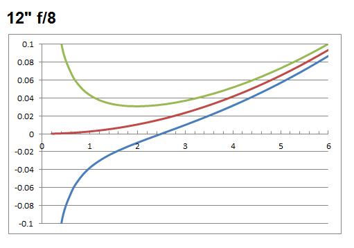
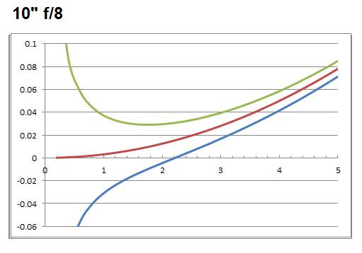
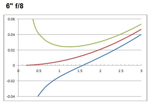
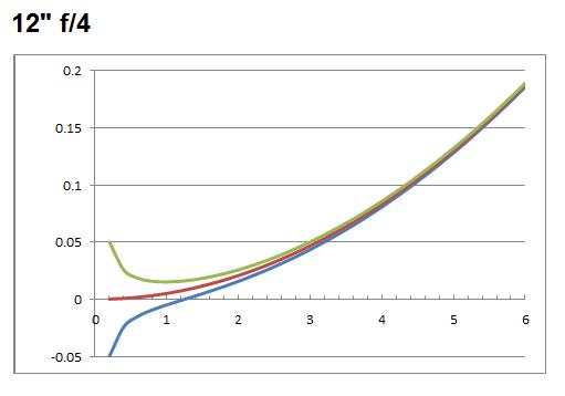
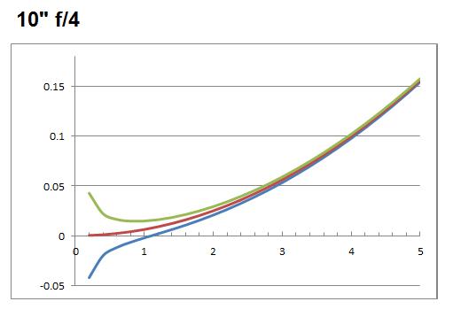
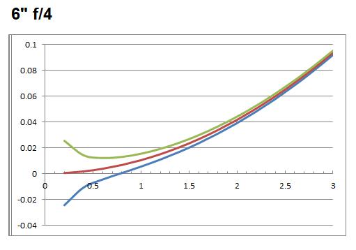
I call this the “tornado” graph because it looks like a sideways tornado. You can see that the errors must be controlled closer on the outer regions than the inner regions. Furthermore, a slow mirror has a fatter tornado than a fast mirror. Slow mirrors are easier to hit the tolerances than a fast mirror. Graph a few to show yourself this fact.

If you plot your points and they are all within this tornado, you can consider yourself finished with your first mirror. The more mirrors you make, the higher degree you will expect from yourself and this will only be a first iteration on your precision. Also, if you plot your points and they all fall within this tornado except for one, then you can slide your points all the same amount up or down together, and if they can all be fit into the tornado, you’re OK.

When you start out with a sphere, the micrometer readings will all be the same, so it will graph a horizontal line. I know I said to start with the center zone and register everybody with respect to it, but what I actually do is start my readings with the outermost zone, work the rest of the zones, then adjust the numbers so they refer to the outermost zone. If my outermost zone is supposed to be 0.612, then I adjust the readings so the outer zone IS 0.612 and see where the others fall. When I graph it at the beginning, all then numbers would be at this outermost zone’s reading, and my horizontal line passes through the top-right point on the tornado and goes horizontally to the left. As I work the mirror, that upper right hand point stays put and the rest of the graph pivots downward. You can see your progress as it pivots until it lands within the tornado everywhere. One reason is that I try to not mess with the outermost regions of the mirror. It has a high amount of area, and getting it goofed up would do the most optical damage, and I like watching my progress as it pivots about that corner.

OK, part 1 of Raleigh’s criteria is that it fits into this tornado [Peak to Valley wave-front error does not exceed ¼ wave]. The second part is the RMS, or root mean square. You can have a rough mirror that fits into the ¼ wave criteria, or you can have a smooth mirror that fits into this criterion. The smooth mirror is better. The second part of his criteria is that the RMS is less than 1/14 wave. To calculate the RMS you must:

0] Make a best-fit model of your data onto your tornado.

1] Determine the distance each reading is from r^2/2R when placed into a best-fit within the tornado.

2] Determine how many eighth waves it is from a perfect curve. The radius of the tornado at each point is an eighth wave on the wave-front.

2] Square each of those distances.

3] Add up all those squares.

4] Divide by how many points you used [4 with a normal Couder mask].

5] Square root the result.

6] Your RMS needs to be less than 1/14 wave.

A note: This needs to be done on more than one axis. You may find that even though there is no first degree astigmatism, you may have differing radii of curvatures for intermediate zones, making it “lumpy”, and this needs to be corrected.

Raleigh’s Criteria says your wave-front error must not exceed ¼ wave and your RMS must not exceed 1/14 wave. If this is true, and there is no TDE, no astigmatism, you have a finished mirror. Again, as you make better and better mirrors, you will increase your personal standards and the Foucault test will no longer be sufficient.

One question that arises is what do you do if the edge is good, the center is good, but an intermediate zone is high or low? With sub-diameter laps, you can “anti-correct”, or “lift” a zone by doing chordal strokes. If your 71% zone is too low [too deep, too concave, too short ROC], you can run strokes through the 71% zone with chordal strokes which will flatten that area [increasing its ROC] as well as shortening the ROC at the endpoints of that stroke. If your intermediate zone is too long, you can shorten them by doing chordal strokes that end at that zone. If your 71% zone is too long, then a chordal stroke that begins at the 71% zone on your side and to the right and ends at the 71% zone on the far side and one the right will deepen the 71% zone while only blending the intermediate region between the endpoints.

Click ME to see a You Tube video of correcting a zone.

You now have a way to add correction, remove correction, at any place on the mirror, and can eventually place all the points on the mirror at their correct ROCs. After correcting zones you may have to smooth out troughs of work, and this can be done by smooth and slow W strokes over the whole mirror with a small lap which ought to not add or remove any correction, but should blend out the ripples.

Let’s run through an example mirror!

Consider a 10” mirror whose center has a radius of curvature of 112.7”. That means the focal length is half of 112.7, or 56.35”, making the telescope an f/5.64 optic.

R = 112.7, 2R = 125.4”, r =1.22 * 0.00055 * 5.635 / 25.4 inches = 0.000014886 inches. This is the radius of the Airy disk. Rr = 112.7 * 0.000014886 = 0.01678.

Let’s let the zones be the same ratios of the diameter as the 8” mirror exampled by Jean Texereau on page 82 of his American 2^nd edition of “How to Make a Telescope”. His 8” couder mask radii are

z1: 0.708, z2: 1.988, z3: 2.948, z4: 3.648 inches

Proportioning those to a 10” mirror, our radii would be

Z1: 0.885”

Z2: 2.485”

Z3: 3.685”

Z4: 4.56”

We need the following columns on our shear sheet: Zones, Radii, , , , and .

Here it is:

Zone	Radius
1	0.885	0.006	0.019	-0.013	0.025
2	2.485	0.049	0.007	0.042	0.056
3	3.685	0.108	0.005	0.103	0.113
4	4.56	0.166	0.004	0.162	0.170

This means that we have for zone 1 a range from -0.013 through 0.025 for our acceptable adjusted micrometer readings, from 0.042 through0.056 for zone 2, 0.103 through 0.113 for zone 3, and 0.162 through 0.170 for zone 4. It’s time to measure the radii of curvature for these zones. We now set the mirror onto the test stand, and set up or Foucault tester so t hat when we look past the razor we an see the mirror illuminated by the test light. We move it around so that when the razor, when moved laterally, intercepts that light it tries to blank out the mirror not from the left, not form the right, but altogether uniformly. It won’t because we’ve worked the mirror, so some of it will darken on the right and some of it will darken on the left. It ought to look a bit like a doughnut lit form the side. Once at the point, we can place the Couder mask onto the mirror. It has holes on it whose centers are at the radii on our chart. We adjust the axial micrometer so that the position of the light and razor allow the outermost zone, zone 4, to black out on the right side at the same moment it blacks out on the left side. When we have accomplished this, we read the micrometer position. Let’s pretend that the micrometer is reading 0.684. We record this. Now we move the razor and light inward toward the mirror by leaving the test stand stationary but rolling the micrometer in until when we move the razor side to side the two zone 3 holes black out simultaneously. We then record this micrometer reading. Let’s pretend that this time it reads 0.629. We then do this for zone 2, and let’s pretend that we get 0.559, and finally let’s use for zone 1 0.508.

There we go, we have readings. Normally, we would repeat this numerous times to make sure the numbers are repeatable, average them up, and perform this on multiple axes. But for now, let’s run the numbers.

Here is our new data sheet.

Zone	Radius					Actual readings	Adjusted readings
1	0.885	0.006	0.019	-0.013	0.025	0.508	-0.008
2	2.485	0.049	0.007	0.042	0.056	0.559	0.043
3	3.685	0.108	0.005	0.103	0.113	0.629	0.113
4	4.56	0.166	0.004	0.162	0.170	0.684	0.168

We took the data from the actual readings and added the same number to each one to get the adjusted readings. You can see that all the data points are in or on the tornado. This means that the first criterion has been met. All the data points show the mirror is within 1/8 wave of the true paraboloid. If we had a data point on the very top and a data point on the very bottom, then we’d be high 1/8 and low 1/8 for a total peak to valley error of 2/8 wave, or ¼ wave. Let’s check the sedond criterion.

Zone1, low 14/19 of 1/8 wave, or -0.09 wave. Zone2, low 6/7 of 1/8 wave, or -0.11. Zone3, high 5/5 of 1/8 wave, or +0.13. Zone4, high 2/4 of 1/8 wave, or 0.06.

So our errors in waves are -0.09, -0.11, +0.13, and +0.06. Their average is -0.0025. Their distances from the average are 0.0875, 0.1075, 0.1325, and 0.0625. These differences squared are 0.007656, 0.011556, 0.017556, and 0.003906. The sum of these squares are 0.040674. Divided by 4 is 0.0101685, and the square root of that is 0.1008. This is about 1/10 wave RMS, too big for our criterion. The mirror is not yet finished and needs to be corrected. There is too much correction in the inner part of the mirror, both zones 1 and 2 are too low, and zone 3 is high and needs correcting. So even though the quarter wave peak to valley criterion is met, the fourteenth wave RMS criterion is not met.

Click to get to Ronchi testing